P2D Model Study Notes · Part 3: Butler-Volmer Kinetics

Date: 2026-05-26
Task: Understand and implement the SPM Butler-Volmer equation (electrochemical reaction kinetics)
Progress: BV kinetics · physical intuition + mathematical derivation + code implementation ✓
Learning method: Guided Q&A (question → self-think → hand-derive → reveal answer)

Learning Method

This chapter uses guided learning: each knowledge point starts with a question, allows you to derive yourself, then confirms the answer. When stuck, pause and break it down. All figures generated with matplotlib as PNG.

This chapter is split into three sub-sessions:

Session	Topic	Core Activity	Output
3.1	Physical Intuition	Q&A: overpotential concept → BV forward equation → j₀ dependence → parameter effects	`linear_approximation.png`
3.2	Mathematical Derivation	Hand-derive arcsinh inversion → linear approximation → Newton iteration	`newton_bv_iteration.png`
3.3	Code Implementation	Build BV function from scratch → visualize → compare with model.py	`bv_my.py` + `bv_overpotential.png`

BV Equation in the SPM Pipeline

Current i_app
    ↓
Flux j = i_app / (a_s·L·F)     ← Chapter 1 knowledge
    ↓
BV equation → Overpotential η            ← This chapter
    ↓        ↑
c_s_surf  (from diffusion equation)       ← Chapter 2 completed
    ↓
V_cell = U_p + η_p − U_n − η_n   ← Chapter 4 implementation

Diffusion (Chapter 2) answers “how lithium distributes inside the particle”, BV (this chapter) answers “how difficult the surface reaction is”. Together → compute overpotential → voltage deviates from ideal OCV.

Session 3.1: Physical Intuition — From “Customs” to the BV Equation

3.1.1 Why Does Overpotential Exist?

Lithium ions entering a graphite particle from the electrolyte is a charge transfer reaction:

$$\text{Li}^+{\text{(electrolyte)}} + e^-{\text{(anode)}} \rightleftharpoons \text{Li}_{\text{(graphite)}}$$

This reaction is not just “drift across and done”. It requires:

Desolvation: Li⁺ in the electrolyte is wrapped in solvent molecules; it must first shed its solvent shell
Crossing the interface energy barrier: Bare Li⁺ crosses the electrolyte/solid interface — this is the core step described by the BV equation
Receiving an electron: Li⁺ + e⁻ → Li (reduction)

Analogy	Customs
Has a visa (OCV says entry is allowed)	Thermodynamic driving force exists
Customs queue	Interface energy barrier = kinetic resistance
Time spent in queue	Overpotential η

Key insight: Higher barrier → harder reaction → same current needs larger η. The BV equation describes this “extra push”.

3.1.2 Equilibrium — Dynamic Balance

At equilibrium (η=0):

         Forward reaction v_fwd
Li⁺(electrolyte) ──────────→ Li(graphite)
          ←──────────
         Reverse reaction v_bck

v_fwd = v_bck = j₀ (exchange current density)
Net current j = v_fwd − v_bck = 0

Key insight: At η=0, both directions react at high speed microscopically (j₀ measures “how busy microscopically”), just at equal rates. Larger j₀ → a small voltage produces large net current → good battery.

3.1.3 Sign Convention of Overpotential

Electrode	Reaction during discharge	η sign	Meaning
Anode	Deintercalation (oxidation)	η_n > 0	Oxidation overpotential
Cathode	Intercalation (reduction)	η_p < 0	Reduction overpotential

Voltage formula verification (Chapter 4 preview):

$$V_{cell} = U_p + \eta_p - U_n - \eta_n = OCV - |\eta_p| - |\eta_n|$$

Overpotential is a “deduction” — discharge voltage is always lower than ideal OCV.

3.1.4 Exchange Current Density j₀

At α=0.5:

$$j_0 = k \cdot \sqrt{c_e} \cdot \sqrt{c_s} \cdot \sqrt{c_{\mathrm{max}} - c_s}$$

Factor	Physical Meaning	Intuition
k	Reaction rate constant	“Entry barrier” height
√c_e	Electrolyte lithium concentration	“Supply” side
√c_s	Surface solid-phase concentration	“How much lithium can leave”
√(c_max−c_s)	Available vacancies	“How many slots can accept”

Key insight: j₀ ∝ √x·√(1−x) (x=SOC), maximum at SOC=50%. At SOC=0, no lithium to deintercalate; at SOC=100%, no vacancies to accept — j₀ approaches 0 at both ends.

3.1.5 Effect of k on Battery Performance

k↑10× → j₀↑10× → j/(2j₀)↓10× → arcsinh(smaller number) → η↓.

Parameter	Impact chain	Conclusion
k↑	→ j₀↑ → η↓ → internal resistance↓	Goal of materials science: find materials with large k

3.1.6 Key Parameter Quick Reference

Parameter	Value	Meaning
k_n, k_p	2.0×10⁻¹¹	Reaction rate constants
c_e	1000 mol/m³	Electrolyte concentration (constant in SPM)
alpha	0.5	Symmetry factor
c_s_max_n	31507 mol/m³	Anode maximum concentration
c_s_max_p	51554 mol/m³	Cathode maximum concentration
T	298.15 K	Temperature
F	96485 C/mol	Faraday constant
R	8.314 J/(mol·K)	Ideal gas constant
RT/F	0.02569 V	Thermal voltage (linear region scale)

Session 3.2: Mathematical Derivation — From BV Forward to arcsinh Inversion

3.2.1 BV Forward Equation

General form:

$$j = j_0 \cdot \left[ \exp!\left(\frac{\alpha F \eta}{RT}\right) - \exp!\left(-\frac{(1-\alpha)F \eta}{RT}\right) \right]$$

Substituting α=0.5:

$$j = j_0 \cdot \left[ \exp!\left(\frac{F\eta}{2RT}\right) - \exp!\left(-\frac{F\eta}{2RT}\right) \right]$$

3.2.2 sinh Form

Recall the hyperbolic sine definition:

$$\sinh(x) = \frac{e^x - e^{-x}}{2}$$

Let A = Fη/(2RT), then BV equation = j₀·[e^A − e^(−A)] = 2j₀·sinh(A):

$$j = 2j_0 \cdot \sinh!\left(\frac{F\eta}{2RT}\right)$$

3.2.3 arcsinh Inversion

j = 2j₀ · sinh(Fη/2RT)
j/(2j₀) = sinh(Fη/2RT)
arcsinh(j/(2j₀)) = Fη/(2RT)
η = (2RT/F) · arcsinh(j/(2j₀))

Step	Operation
1	Divide both sides by 2j₀
2	Take arcsinh of both sides
3	Multiply both sides by 2RT/F

$$\eta = \frac{2RT}{F} \cdot \mathrm{arcsinh}!\left(\frac{j}{2j_0}\right)$$

Numerical verification (2RT/F ≈ 51.4 mV, T=298.15K):

j/(2j₀)	arcsinh	η
1.0	0.881	45.3 mV
0.1	0.0998	5.1 mV

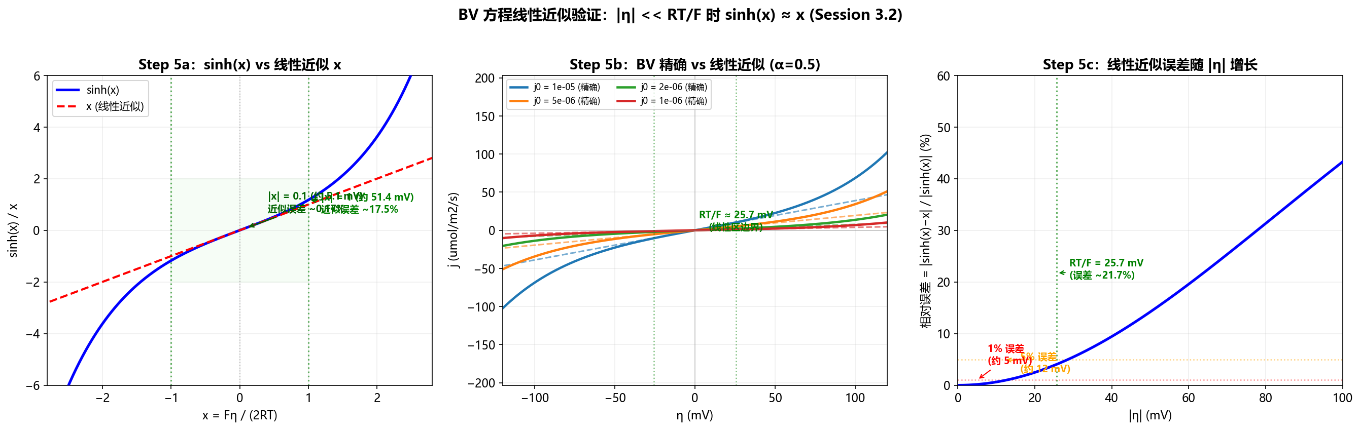
3.2.4 Small-η Linear Approximation

Taylor expansion of sinh(x):

$$\sinh(x) = x + \frac{x^3}{6} + \frac{x^5}{120} + \cdots$$

When |x| ≪ 1: sinh(x) ≈ x.

Substituting: j ≈ 2j₀·Fη/(2RT) = j₀·Fη/(RT), inverting:

$$\eta \approx \frac{RT}{F} \cdot \frac{j}{j_0} \quad\quad (|\eta| \ll RT/F)$$

| |η| Range | Error | Applicable Scenario |
|——|——|——|
| < 5 mV | ~0.2% | Small current (below C/5) |
| < 25.7 mV (RT/F) | ~21.7% | Medium current |
| > 50 mV | > 55% | ❌ Must use arcsinh |

Physical meaning: η = R_ct·j, where R_ct = RT/(F·j₀) is the charge transfer resistance — at small current, BV reduces to Ohm’s law.

3.2.5 Why α≠0.5 Cannot Use arcsinh?

At α≠0.5, the two exponentials are asymmetric:

	α=0.5	α=0.3
Exp 1	exp(0.5A)	exp(0.3A)
Exp 2	exp(−0.5A)	exp(−0.7A)
Symmetric?	Yes → sinh	No → no analytic solution

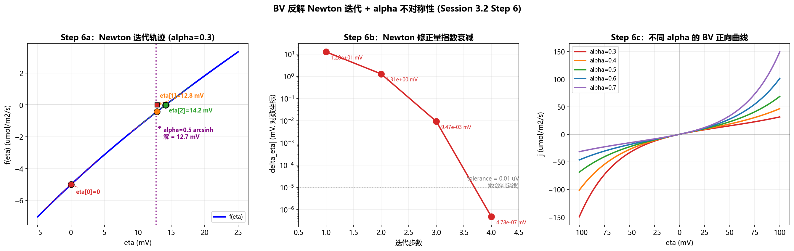
3.2.6 Newton Iteration

Define the residual function:

$$f(\eta) = j_0 \cdot \left[ e^{\alpha F\eta/RT} - e^{-(1-\alpha)F\eta/RT} \right] - j$$

Newton formula:

$$\eta_{\text{new}} = \eta_{\text{old}} - \frac{f(\eta_{\text{old}})}{f’(\eta_{\text{old}})}$$

Geometric meaning: Draw tangent at current point → tangent’s x-axis intersection = next guess → repeat.

Convergence speed: Quadratic convergence — significant digits double each step. Starting from η=0, converges to nanovolt precision within 3 steps.

Algorithm logic (model.py lines 238–253):

Algorithm: newton_bv_inversion(j, j₀, α, T)
  Initialize: η = 0
  For iteration 1..20:
    1. Compute A = F·η / (R·T)
    2. Compute residual: f = j₀·[exp(α·A) − exp(−(1−α)·A)] − j
    3. Compute derivative: f' = j₀·(F/(R·T))·[α·exp(α·A) + (1−α)·exp(−(1−α)·A)]
    4. Compute correction: dη = −f / max(f', 1e⁻²⁰)
    5. Update: η = η + dη
    6. If |dη| < 1e⁻⁸: converged → break
  Return η

Session 3.3: Code Implementation — Independent Implementation + Visualization + Verification

3.3.1 Core Formulas (α=0.5)

1 2	j₀ = k · c_e^0.5 · c_s_surf^0.5 · (c_max − c_s_surf)^0.5 η = (2RT/F) · arcsinh(j / (2·j₀))

3.3.2 Defensive Programming

Issue	Solution
c_s_surf = 0 or c_s_max → j₀ = 0 → division by zero	`np.clip(c_s_surf, 1e-12, c_s_max − 1e-12)`
j/(2j₀) too large → arcsinh overflow	`np.clip(j/(2*j₀), -1e10, 1e10)`

3.3.3 Independent Implementation: bv_my.py

Function: bv_overpotential(j, k, c_e, c_s_surf, c_s_max, alpha, T)
  Purpose: Compute overpotential η from current density j via Butler-Volmer inversion

  Constants: F = 96485.0, R = 8.314

  Algorithm:
    1. Clip c_s_surf to [1e⁻¹², c_s_max − 1e⁻¹²] to prevent j₀ = 0
    2. Compute exchange current density:
       j₀ = k · c_e^(1−α) · c_s_surf^α · (c_max − c_s_surf)^(1−α)
    3. If α = 0.5:
       a. Compute argument: x = clip(j / (2·j₀), −1e¹⁰, 1e¹⁰)
       b. Return η = (2RT/F) · arcsinh(x)
    4. Else (α ≠ 0.5, Newton iteration):
       a. Initialize η = 0
       b. Loop (max 20 iterations):
          · Compute A = F·η / (R·T)
          · Compute residual: f = j₀·[exp(α·A) − exp(−(1−α)·A)] − j
          · Compute derivative: f' = j₀·(F/(R·T))·[α·exp(α·A) + (1−α)·exp(−(1−α)·A)]
          · Compute correction: dη = −f / max(f', 1e⁻²⁰)
          · Update: η += dη
          · If |dη| < 1e⁻⁸: break (converged)
       c. Return η

  Returns: η (overpotential in volts)

3.3.4 Verification Result

1
2
3

my_bv:   −2.630587 mV
ref_bv:  −2.630587 mV
diff:    0.000 nV    ← Exact match

3.3.5 Generated Visualizations

Figure	Content
linear_approximation.png	sinh(x) vs x comparison · j-η linear approximation · error growth
newton_bv_iteration.png	Newton iteration trajectory · correction decay · α asymmetry
bv_overpotential.png	η→j (different SOC) · j→η (arcsinh) · j₀ vs SOC

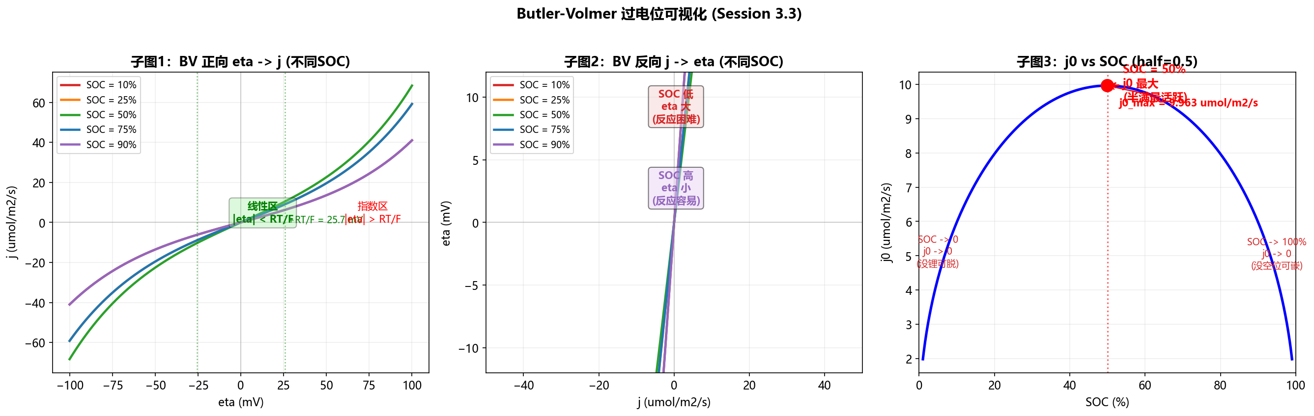
3.3.6 Interpreting the Three Subplots of bv_overpotential.png

Subplot 1: BV Forward η→j

Observation	Meaning
Green shaded region (	η
Outside green region	Exponential region, curve rises steeply
SOC=90% (purple) is flattest	j₀ is small → reaction is difficult
SOC=50% (green) is steepest	j₀ is maximum → reaction is easiest

Subplot 2: BV Inverse j→η

Observation	Meaning
SOC=90% (purple) at bottom	For given j, η is smallest → least reaction resistance
SOC=10% (red) at top	For given j, η is largest → most reaction resistance

Subplot 3: j₀ vs SOC

Observation	Meaning
“∩” shape curve	Classic shape of √x·√(1−x)
Maximum at SOC=50%	Equal lithium and vacancies, bidirectional flow is smoothest
Approaches 0 at both ends	SOC→0 (nothing to deintercalate) or SOC→100% (no vacancies to accept)

File Index

File	Purpose	Status
`session_03_background.md`	Session entry file	✅
`learning_notes_03_kinetics.md`	These notes	✅
`bv_my.py`	Independent BV implementation	✅ 0 nV difference vs model.py
`visualize_linear_approximation.py`	Linear approximation visualization script	✅
`visualize_newton_bv.py`	Newton iteration visualization script	✅
`visualize_bv_overpotential.py`	BV three-subplot visualization script	✅
`linear_approximation.png`	sinh vs x + error growth	✅
`newton_bv_iteration.png`	Newton trajectory + asymmetry	✅
`bv_overpotential.png`	η→j + j→η + j₀ vs SOC	✅
`../../spm/model.py`	BV function source (butler_volmer_overpotential)	Reference
`../../spm/parameters.py`	Battery parameters	Reference

Connection to Adjacent Chapters

┌──────────────┐     c_s_surf     ┌──────────────┐      eta      ┌──────────────┐
│  Chapter 2   │ ──────────────→ │  Chapter 3   │ ───────────→ │  Chapter 4   │
│  Diffusion   │                 │  BV Kinetics │              │  Full SPM    │
│  Fick's Law  │                 │              │              │  Voltage     │
│              │  ←────────────  │              │              │              │
│  Update c(r) │       j         │  Output η    │              │ V=U+η_p+η_n  │
└──────────────┘                 └──────────────┘              └──────────────┘

Preview Questions (Before Entering Chapter 4)

Is OCV + η equal to the battery voltage? Are there other “deductions”?
How are the four SPM equations (OCV, BV, diffusion, voltage coupling) chained together in model.py’s step()?
If you had to write a step() function from scratch, what inputs do you need? What does it output?

Understand the physical meaning of overpotential
Master the BV forward equation and j₀ dependence
Hand-derive the α=0.5 arcsinh inversion
Understand the small-η linear approximation and its range of validity
Understand the Newton iteration solution approach
Independently implement bv_overpotential() function
Plot η-j curves and j₀ dependence graphs
Compare independent implementation vs model.py (0 nV difference)

End of Notes · Next: Full SPM Implementation & Voltage Coupling