P2D Model Study Notes · Part 1: Fundamental Concepts & OCV
Date: 2026-05-21
Task: Build an electrochemical battery simulation model from scratch in Python
Progress: SPM Single Particle Model · OCV Curves Complete
1. What Can Electrochemical Simulation Do?
Electrochemical simulation = creating a “digital twin” of a battery — using mathematical equations to simulate everything happening inside a battery on a computer.
| What You Want to Know | What Simulation Can Tell You |
|---|---|
| How much charge remains? | Simulate how voltage drops during discharge |
| How much current can it handle? | Simulate whether the battery interior “congests” under different currents |
| Why does the battery heat up? | Simulate internal losses → heat generation |
| How long will the battery last? | Simulate aging processes (cycle life) |
| How to design better batteries? | Adjust parameters and observe performance changes |
2. What Happens Inside a Li-ion Battery?
Three key steps during discharge:
1 | graph LR |
- Deintercalation: Lithium atoms at the anode particle surface lose electrons, becoming Li⁺ that enter the electrolyte
- Migration: Li⁺ travels through the electrolyte (separator) toward the cathode
- Intercalation: Li⁺ gains electrons at the cathode particle surface and embeds into the cathode
3. What is SPM (Single Particle Model)?
SPM = Single Particle Model, the simplest electrochemical battery model.
1 | graph TD |
Three Core Assumptions of SPM
| Assumption | Meaning |
|---|---|
| (1) All particles behave identically | One sphere represents the entire electrode |
| (2) Neglect electrolyte concentration variations | Li⁺ concentration is uniform throughout the electrolyte |
| (3) Uniform current distribution | Each particle experiences the same current |
SPM Capability Boundaries
- Voltage–time curves (discharge/charge curves)
- Lithium concentration distribution within particles
- Battery performance under different currents
- SOC evolution over time
- Accurate prediction at high currents (neglects electrolyte gradients)
- Differences between particles at different positions
4. Parameter Naming Convention
Naming formula: self.{quantity}_{phase}_{position}
Quantity Prefixes
| Prefix | Meaning | Common Units |
|---|---|---|
L |
Length / Thickness | m |
R |
Radius or Ideal Gas Constant | m / J·mol⁻¹·K⁻¹ |
c |
Concentration | mol·m⁻³ |
D |
Diffusion Coefficient | m²·s⁻¹ |
eps |
Volume Fraction / Porosity | Dimensionless |
k |
Reaction Rate Constant | Context-dependent |
i |
Current Density | A·m⁻² |
F |
Faraday Constant | 96485 C·mol⁻¹ |
T |
Temperature | K |
Nr |
Number of Discrete Points | Dimensionless |
Phase Suffixes & Position Suffixes
| Suffix | Category | Meaning |
|---|---|---|
_s |
Phase | Solid Phase |
_e |
Phase | Electrolyte Phase |
_n |
Position | Negative Electrode |
_p |
Position | Positive Electrode |
_s |
Position | Separator |
Note:
_scan denote either “solid phase” or “separator” depending on context. For example,eps_s_n= negative solid-phase volume fraction,eps_e_s= separator electrolyte volume fraction.
Combination Examples
| Variable Name | Decomposition | Meaning |
|---|---|---|
c_s_max_n |
c + s + max + n | Maximum lithium concentration in negative solid phase |
D_s_p |
D + s + p | Positive solid-phase diffusion coefficient |
eps_e_s |
eps + e + s | Separator electrolyte volume fraction |
i_app |
i + app(applied) | Applied current density |
5. Cell SOC vs. Electrode SOC
Key Distinction
Cell SOC ≠ a given electrode’s SOC. During discharge, the two electrodes evolve in opposite directions:
| Negative SOC | Positive SOC | |
|---|---|---|
| Cell 100% (Full) | 95% | 10% |
| Cell 0% (Empty) | 5% | ~79% |
| Direction (Discharge) | ↓ Decreasing | ↑ Increasing |
SOC Relationship Governed by Lithium Conservation
Moles of lithium lost by the anode = Moles of lithium gained by the cathode:
$$
N_{\mathrm{total}} \cdot \Delta SOC_n = P_{\mathrm{total}} \cdot \Delta SOC_p
$$
$$
\frac{\Delta SOC_p}{\Delta SOC_n} = \frac{N_{\mathrm{total}}}{P_{\mathrm{total}}} \quad \text{(SOC Exchange Rate)}
$$
Key insight: This relationship is exactly linear — it is a direct consequence of mass conservation, not an approximation.
N/P Capacity Ratio
$$
N_{\mathrm{total}} = c_{s,\mathrm{max}}^n \cdot \varepsilon_s^n \cdot L_n \cdot A
$$
$$
P_{\mathrm{total}} = c_{s,\mathrm{max}}^p \cdot \varepsilon_s^p \cdot L_p \cdot A
$$
$$
\mathrm{N/P} = \frac{N_{\mathrm{total}}}{P_{\mathrm{total}}}
$$
| N/P Value | Implication |
|---|---|
| > 1 | Anode capacity > Cathode capacity → Cathode is the limiting electrode during charge → Prevents lithium plating |
| < 1 | Cathode capacity > Anode capacity → Anode is the limiting electrode during discharge |
| Does not determine | Initial SOC pairing, but constrains how far discharge/charge can proceed |
Cell-Level SOC → Electrode SOC Automatic Conversion
In parameters.py, simply set battery_soc_initial = 0.3 (cell starts at 30%), and the program computes automatically.
1 | graph TD |
6. OCV Curves (Open-Circuit Voltage)
OCV is the “fingerprint” of an electrode material — each material has a unique OCV–SOC relationship.
6.1 The Nernst Equation (Thermodynamic Foundation)
$$
OCV(\theta) = U_0 + \frac{RT}{F} \cdot \ln!\left(\frac{\theta}{1-\theta}\right)
$$
| Symbol | Name | Value | Meaning |
|---|---|---|---|
| $U_0$ | Reference Potential | ~0.12 V (graphite) / ~3.85 V (NMC) | Characteristic potential of the material |
| $R$ | Ideal Gas Constant | 8.314 J·mol⁻¹·K⁻¹ | |
| $T$ | Temperature | 298.15 K | |
| $F$ | Faraday Constant | 96485 C·mol⁻¹ | |
| $RT/F$ | Thermal Voltage | 0.02569 V | The “thermal ruler” of one electron |
| $\theta$ | Surface SOC | $c_{s,\mathrm{surf}} / c_{s,\mathrm{max}}$ |
Physical Origin: The Nernst equation derives from the Gibbs free energy $\Delta G = \Delta G_0 + RT \cdot \ln(\mathrm{activity\ ratio})$; it generates a complete curve with only 2 parameters. However, it assumes the material is an “ideal solution” — atoms do not interact with each other.
6.2 Ideal vs. Real
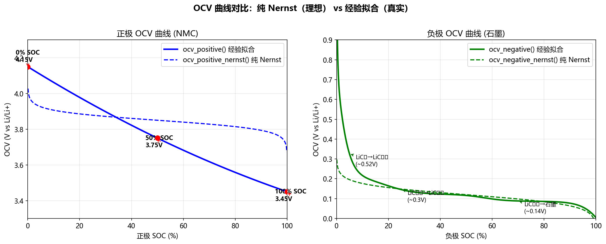
| Ideal Solution (Nernst) | Real Graphite | Real NMC | |
|---|---|---|---|
| Curve Shape | Smooth S-shape | Staircase plateaus | Smooth but asymmetric |
| Cause | No inter-atomic interactions | LiC₆→LiC₁₂→LiC₁₈ phase transitions | Multi-transition-metal synergy |
| Fitting Method | 2 parameters | Nernst + tanh steps | Nernst + polynomial |
6.3 Nernst Equation Breakdown
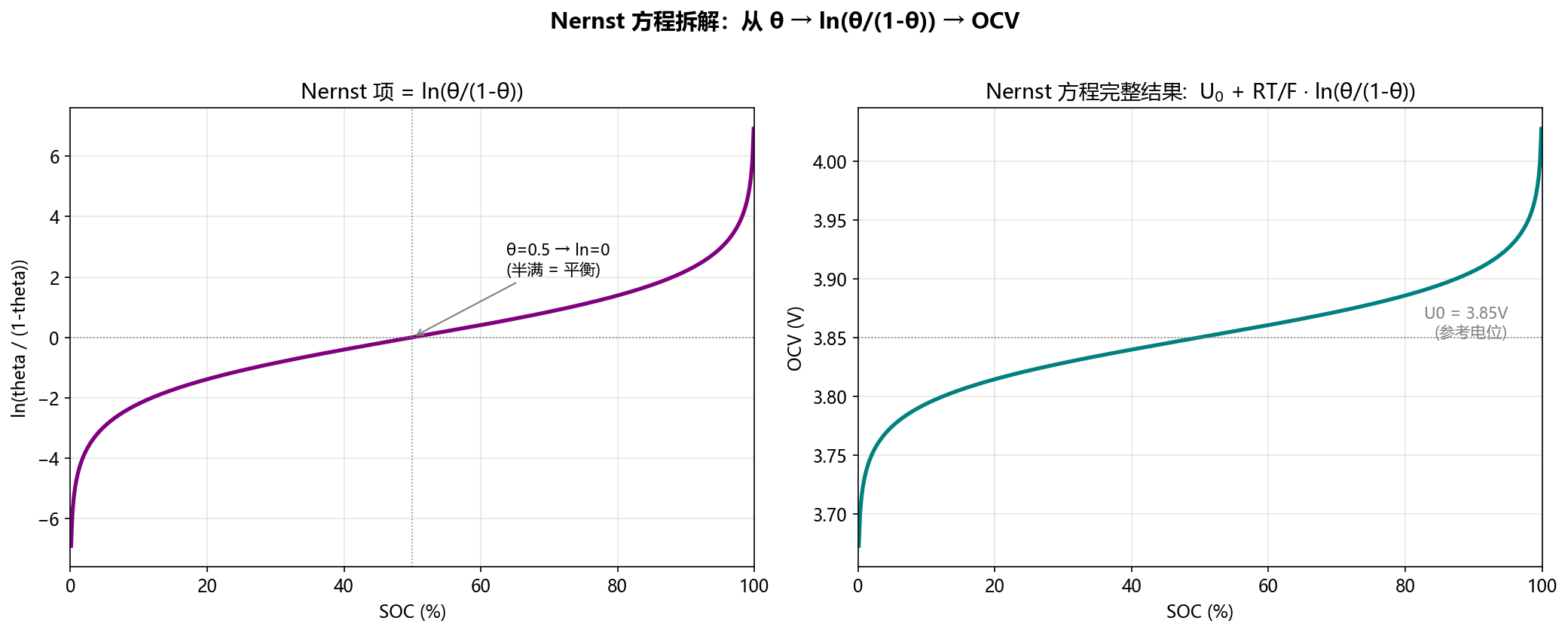
The core of Nernst is simply $\ln(\theta/(1-\theta))$, multiplied by the thermal voltage $RT/F \approx 0.026\mathrm{V}$:
- $\theta = 0.5$: $\ln(1) = 0$, $OCV = U_0$ (equilibrium)
- $\theta \to 0$: $\ln \to -\infty$, OCV drops steeply
- $\theta \to 1$: $\ln \to +\infty$, OCV rises steeply
Key Insight: The “logarithmic scale” is compressed into the “millivolt scale” by the thermal voltage — the shape of the curve is entirely a mathematical expression of the entropy of mixing.
6.4 Graphite Anode OCV (ocv_negative)
1 | def ocv_negative(theta): |
Essentially, mathematical “building blocks” (tanh smooth steps + exp spike) are used to approximate the staircase-like OCV produced by graphite phase transitions:
$$
OCV_{\mathrm{graphite}}(\theta) = \mathrm{constant} + \sum_k a_k \cdot \tanh!\left(\frac{\theta - \theta_k}{w_k}\right) + \mathrm{exp\ term}
$$
Each $\tanh$ step corresponds to one phase-transition stage of graphite during lithiation/delithiation.
6.5 NMC Cathode OCV (ocv_positive)
1 | def ocv_positive(theta): |
$$
OCV_{\mathrm{NMC}}(\theta) = 4.15 - 0.9\theta + 0.2\theta^2
$$
| Control Point | OCV |
|---|---|
| $\theta = 0$ | 4.15 V (fully delithiated, highest potential) |
| $\theta = 0.5$ | 3.75 V (half-full) |
| $\theta = 1$ | 3.45 V (fully lithiated, lowest potential) |
6.6 The Full Picture: Four-Term Superposition
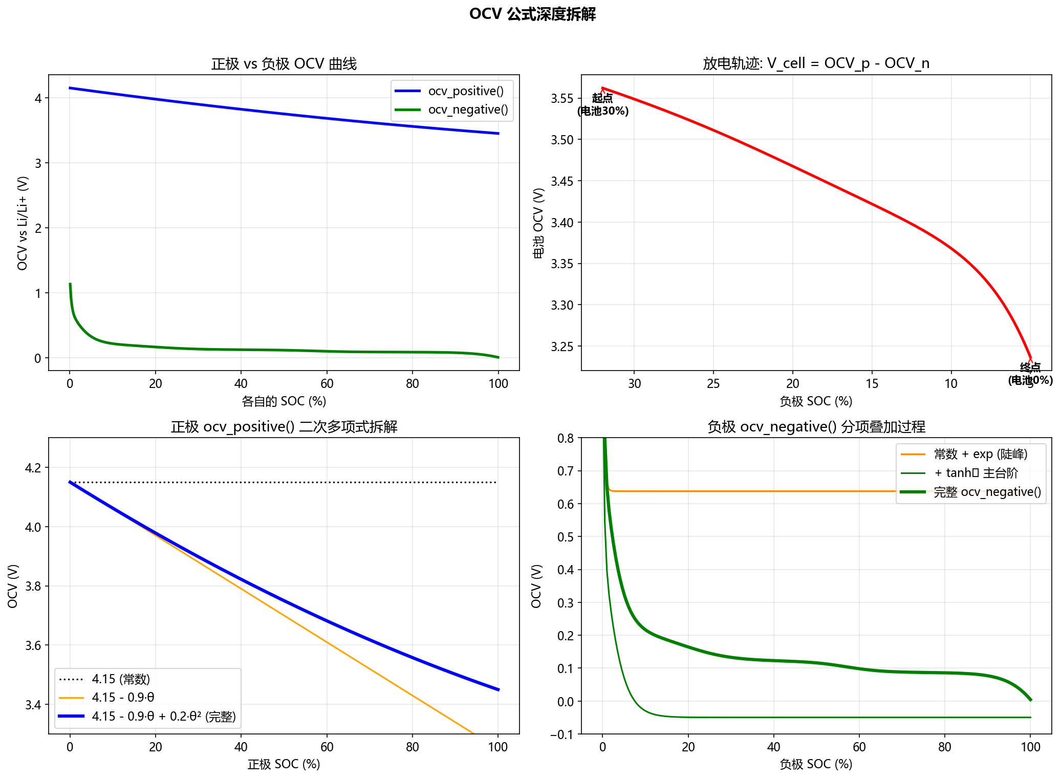
Focus on the upper-right subplot — this is the OCV trajectory when discharging from 30% SOC to 0%:
$$
V_{\mathrm{cell}} = OCV_p(SOC_p) - OCV_n(SOC_n)
$$
From ~3.65 V (start) down to ~3.45 V (end).
Note: This is only the OCV contribution; the overpotential $\eta$ has not been included yet (adding $\eta$ will depress the voltage further).
7. The Four OCV Functions at a Glance
| Function | Type | Purpose |
|---|---|---|
ocv_negative() |
Empirical Fit | Used at runtime, real graphite curve |
ocv_positive() |
Quadratic Polynomial | Used at runtime, real NMC curve |
ocv_negative_nernst() |
Pure Physics | Teaching use, comparing “ideal vs. real” |
ocv_positive_nernst() |
Pure Physics | Teaching use, comparing “ideal vs. real” |
8. The SPM Four-Equation Panorama
1 | graph TD |
9. Project File Structure
1 | c:\Project\P2D\ |
10. Key Formula Quick Reference
| Formula | Meaning |
|---|---|
| $V_{\mathrm{cell}} = OCV_p - OCV_n$ | Cell open-circuit voltage = Cathode potential − Anode potential |
| $\frac{\Delta SOC_p}{\Delta SOC_n} = \frac{N_{\mathrm{total}}}{P_{\mathrm{total}}}$ | SOC exchange rate (lithium conservation) |
| $Q_{\mathrm{Ah}} = \frac{F \cdot \min(cap_n, cap_p)}{3600}$ | Cell capacity [Ah] |
| $i_{1C} = \frac{Q_{\mathrm{Ah}}}{A}$ | 1C current density |
| $j = \frac{i}{a_s \cdot L \cdot F}$ | Current density → reaction flux |
| $a_s = \frac{3 \cdot \varepsilon_s}{R}$ | Active specific surface area (spherical particles) |
| $OCV(\theta) = U_0 + \frac{RT}{F}\ln!\left(\frac{\theta}{1-\theta}\right)$ | Nernst equation |
| $OCV_{\mathrm{NMC}}(\theta) = 4.15 - 0.9\theta + 0.2\theta^2$ | NMC cathode OCV |
11. To-Do / Next Steps
- Understand SPM model concepts
- Master parameter naming rules and physical meanings
- Understand N/P ratio and SOC conversion
- Understand OCV curves (Nernst + empirical fitting)
- Study the diffusion equation (Fick’s Second Law in spherical coordinates)
- Study Butler-Volmer kinetics
- Study voltage coupling
- Write
simulate.py, run a complete simulation - Plot discharge curves, analyze results
End of Notes · Next Part: Diffusion Equation & Butler-Volmer Kinetics