P2D Model Study Notes · Part 2: Diffusion Equation

Date: 2026-05-25
Task: Understand and implement the SPM diffusion equation (Fick’s Second Law in spherical coordinates)
Progress: Diffusion equation · physical intuition + numerical discretization + code implementation ✓
Learning method: Guided Q&A (question → self-think → hand-derive → reveal answer)

Learning Method

This chapter uses guided learning: each knowledge point starts with a question, allows you to derive yourself, then confirms the answer. When stuck, pause and break it down. No plain-text diagrams — all figures generated with matplotlib as PNG.

This chapter is split into three sub-sessions:

Session	Topic	Core Activity	Output
2.1	Physical Intuition	Question → hand-derive Fick’s Second Law → build intuition from figures	`diffusion_concept.png`
2.2	Numerical Methods	Hand-derive Taylor differences, Laplacian discretization, L’Hôpital’s rule, CFL	`diffusion_discretization.png`
2.3	Code Practice	Build diffusion solver from scratch → fix bugs → compare and verify	`diffusion_solver_my.py` + `diffusion_simulation.png`

Session 2.1: Physical Intuition — From “a Cup of Sugar Water” to the Spherical Coordinate Equation

2.1.1 What is Concentration?

Guiding Question: You brewed a cup of coffee and dropped in a sugar cube. When the sugar just settles at the bottom, is the sweetness at the bottom the same as at the top? What about after 10 minutes undisturbed?

Thinking Result: They’re different. Right after dropping, the bottom is sweet, the top is bland. After a long time, it becomes uniform. This is diffusion driven by concentration difference.

Conclusion:

$$
c = \frac{n}{V} \quad [\mathrm{mol/m^3}]
$$

where n = amount of substance (mol), V = volume (m³).

In a battery particle, high c = high SOC (lithium is full), low c = low SOC (lithium is almost gone).

2.1.2 Fick’s First Law — What Pushes the Sugar Molecules?

Guiding Question: Sugar moves from the bottom to the top of the cup — what force is “pushing” it? Is it a special kind of force?

Thinking Result: It’s not a force. Purely random thermal motion + probability. More sugar molecules at the bottom → probabilistically, more sugar molecules “happen” to move from bottom to top. Macroscopically, high concentration flows to low concentration.

Formula:

$$
J = -D \cdot \frac{\partial c}{\partial r}
$$

Symbol-by-symbol breakdown:

Symbol	Name	Intuition	Unit
J	Diffusion flux	Moles passing per second per square meter	mol/(m²·s)
D	Diffusion coefficient	How fast lithium “walks” in this material	m²/s
∂c/∂r	Concentration gradient	How steep the concentration “slope” is	mol/m⁴
−	Negative sign	Ensures correct direction: high → low	—

Actual D values:

Material	D (m²/s)	Intuitive feel
Graphite (negative)	~4×10⁻¹⁴	Very slow, like swimming in honey
NMC (positive)	~1×10⁻¹³	Slightly faster, like swimming in water
Electrolyte	~1×10⁻¹⁰	Much faster, like walking in air

Key insight: Larger D → faster diffusion → concentration non-uniformity recovers to uniformity faster → better battery rate performance.

2.1.3 Fick’s Second Law — Hand-Derive from Mass Conservation

Guiding Question: Fick’s First Law tells us the diffusion speed J, but “how does the concentration c at a given position change over time”?

Learning method: Prepare pen and paper. Derive each step yourself before reading the answer.

Step 1: Take a thin slice inside the particle (thickness dr, cross-sectional area A). Mass conservation —

Write: concentration change in the slice = inflow − outflow

Answer:

$$
\frac{\partial c}{\partial t} \cdot (A \cdot dr) = J(r) \cdot A - J(r+dr) \cdot A
$$

Step 2: Cancel A on both sides, divide by dr. As dr→0, [J(r) − J(r+dr)]/dr = ?

Write the simplified result.

Answer:

$$
\frac{\partial c}{\partial t} = -\frac{\partial J}{\partial r}
$$

Intuition check: if J(r) > J(r+dr) (inflow > outflow), −∂J/∂r > 0, concentration increases ✓

Step 3: Substitute Fick’s First Law J = −D·∂c/∂r.

Write the final result.

Answer — Fick’s Second Law in Cartesian coordinates:

$$
\frac{\partial c}{\partial t} = D \cdot \frac{\partial^2 c}{\partial r^2}
$$

Intuition for ∂²c/∂r²: if the curve is “concave up” (∂²c/∂r² > 0), this point is more dilute than its neighbors → neighbors diffuse in → concentration rises. If “concave down” (∂²c/∂r² < 0), this point is more concentrated than its neighbors → diffuses out → concentration drops.

2.1.4 Spherical Coordinate Correction — The Onion Model

Guiding Question: Battery particles are spherical. Look at the figure subplot 2 (onion model) — are the volumes of the innermost and outermost shells equal?

See figure: diffusion_concept.png middle subplot.

Answer: Shell volume = 4πr²·dr. For shells of equal thickness, volume near center ≈ 0, maximum near surface. So the same amount of lithium entering near the center produces a more dramatic concentration change — like a funnel, the narrower toward the tip, the faster the water level rises.

Fick’s Second Law in spherical coordinates (the derivation is too complex; accept the result for now):

$$
\frac{\partial c}{\partial t} = D \cdot \left[ \frac{\partial^2 c}{\partial r^2} + \frac{2}{r} \cdot \frac{\partial c}{\partial r} \right]
$$

	Cartesian	Spherical
What’s extra	—	+ (2/r)·∂c/∂r
Meaning	—	Geometric focusing effect — closer to center, larger this term becomes

2.1.5 Two Boundary Conditions

Guiding Question 1: At the particle center r=0, in which direction should lithium diffuse? Is there a “preferred” direction?

Thinking Result: The center is perfectly symmetric — up/down/left/right/front/back are all the same. No preferred direction, so ∂c/∂r|₀ = 0 (concentration profile is flat at the center).

Guiding Question 2: During discharge, what is happening at the negative electrode particle surface? Is lithium entering or leaving?

Thinking Result: Recall Course 1: during discharge the negative electrode deintercalates lithium, lithium leaves from the particle surface (j < 0). Fick’s First Law D·∂c/∂r = j, so ∂c/∂r < 0 — surface concentration is lower than interior.

Surface boundary:

$$
D \cdot \frac{\partial c}{\partial r}\bigg|_{r=R} = j
$$

Situation	Sign of j	Surface c vs. Interior
Discharge (negative)	j < 0	c_surf < c_inner
Discharge (positive)	j > 0	c_surf > c_inner
Rest	j = 0	c uniform

See figure subplot 3 (right side): blue gradient from dark interior to light surface, red arrow = deintercalation direction, green arrow = diffusion replenishment direction. This is the physical picture of concentration polarization.

2.1.6 Analogy — Spherical Sponge Squeezing

Guiding Question: If the diffusion coefficient D approaches infinity (water flows infinitely fast), what happens to the interior as water is squeezed from the surface? Does concentration polarization still exist?

Thinking Result: D→∞ means interior water instantly replenishes the surface, concentration remains uniform everywhere, polarization vanishes. Smaller D → surface dries out while interior is still wet → more severe concentration polarization.

Sponge	Battery Particle
Water concentration	Lithium concentration c
Pore size (water flow speed)	Diffusion coefficient D
Squeezing water from surface	Discharge deintercalation (j < 0)
Surface dry, interior wet	Concentration polarization

Key insight: The diffusion equation is the first step moving battery modeling from “statics” to “dynamics”. OCV only tells me “what voltage the battery should have”, diffusion tells me “because lithium can’t diffuse fast enough, actual voltage is lower than the ideal value”.

2.1.7 Session 2.1 Outputs

✅ diffusion_concept.png (three subplots: concentration gradient + onion model + discharge distribution)
✅ Hand-derived Fick’s Second Law (Cartesian form)

Extended Thinking (preview for Session 2.2)

Computers only do addition, subtraction, multiplication, and division — how to compute ∂c/∂r? Hint: slope between two points
At the center r=0, (2/r)·∂c/∂r → 0/0 — how to handle this? Hint: L’Hôpital’s rule

Session 2.2: Numerical Methods — From Finite Differences to Tridiagonal Matrix

2.2.0 Warmup: Two Leftover Questions from Last Session

User feedback: Couldn’t solve the two extended thinking questions.

Question 1: How does a computer compute ∂c/∂r?

You have arrays c[0], c[1], c[2]… The simplest idea — slope between two points: (c_{i+1} − c_i) / dr.

Question 2: How to handle 0/0 at r=0?

L’Hôpital’s rule: differentiate numerator and denominator with respect to r. (2·∂c/∂r)/r → (2·∂²c/∂r²)/1 = 2·∂²c/∂r².

2.2.1 Spatial Discretization — Slicing the Particle into Points

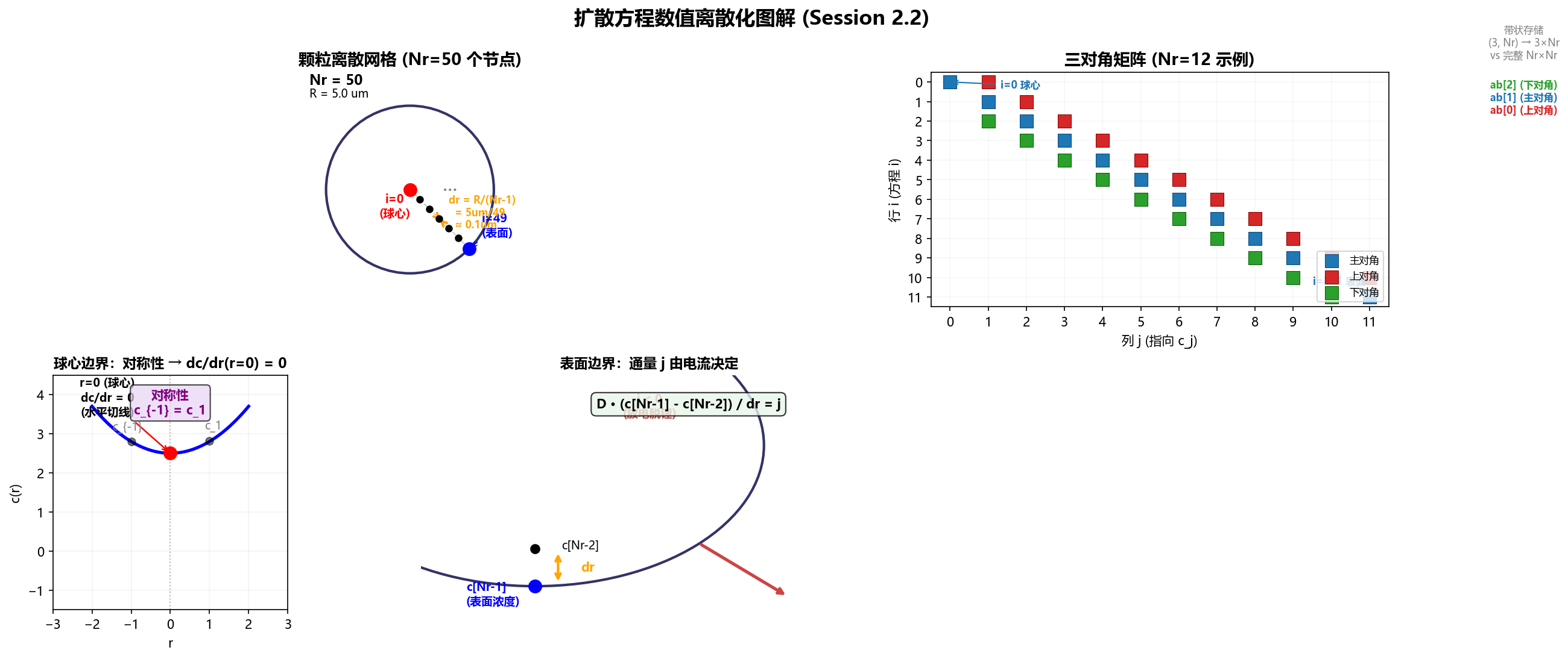
Guiding Question: Particle radius R=5μm, uniformly place Nr=50 points. dr=? Where is i=0? Where is i=49?

Calculation: dr = R/(Nr−1) = 5μm/49 ≈ 0.102μm. i=0 is at the center (r=0), i=49 is at the surface (r=R).

See figure: diffusion_discretization.png upper-left subplot — center red dot (i=0), surface blue dot (i=49), intermediate black dots, orange dr annotation.

The continuous function c(r) becomes the array c[0], c[1], …, c[49].

2.2.2 Taylor Expansion → Finite Difference Hand-Derivation

Taylor expansion: take a small step h forward —

$$
f(x+h) = f(x) + h \cdot f’(x) + \frac{h^2}{2} \cdot f’’(x) + \frac{h^3}{6} \cdot f’’’(x) + \cdots
$$

Derive the first derivative: replace h with −h, subtract f(x−h) from f(x+h), cancel the h² term. Please write it out.

Answer:

$$
f(x+h) - f(x-h) = 2h \cdot f’(x) + \cdots
$$

(The omitted terms are h³ and higher order, negligible since h is small)

$$
f’(x) \approx \frac{f(x+h) - f(x-h)}{2h}
$$

Derive the second derivative: add f(x+h) and f(x−h), cancel the f’ term. Please write it out.

Answer:

$$
f(x+h) + f(x-h) = 2f(x) + h^2 \cdot f’’(x) + \cdots
$$

(The omitted terms are h⁴ and higher order)

$$
f’’(x) \approx \frac{f(x+h) - 2f(x) + f(x-h)}{h^2}
$$

Translating to our notation (h → dr):

$$
\frac{\partial c}{\partial r}\bigg|i \approx \frac{c{i+1} - c_{i-1}}{2 \cdot dr}
\qquad
\frac{\partial^2 c}{\partial r^2}\bigg|i \approx \frac{c{i+1} - 2c_i + c_{i-1}}{dr^2}
$$

2.2.3 Spherical Laplacian Discretization ⭐ Core Derivation

Recall spherical coordinates: ∇²c = ∂²c/∂r² + (2/r)·∂c/∂r.

Please substitute both difference formulas and combine like terms.

After substitution:

$$
\nabla^2 c_i = \frac{c_{i+1} - 2c_i + c_{i-1}}{dr^2} + \frac{2}{r_i} \cdot \frac{c_{i+1} - c_{i-1}}{2 \cdot dr}
$$

Simplify the second term: (2/r_i) × 1/(2dr) = 1/(r_i·dr):

$$
\nabla^2 c_i = \frac{c_{i+1} - 2c_i + c_{i-1}}{dr^2} + \frac{c_{i+1} - c_{i-1}}{r_i \cdot dr}
$$

Combine the c_{i-1} coefficient:

$$
\frac{1}{dr^2} - \frac{1}{r_i \cdot dr}
$$

User got stuck: “I don’t understand this step.”

Breakdown — this is basic fraction combination. Extract common factor 1/dr²:

Convert the second fraction 1/(r_i·dr) to denominator dr²: multiply numerator and denominator by dr → dr/(r_i·dr²) = (dr/r_i)/dr². Therefore:

$$
\frac{1}{dr^2} - \frac{dr/r_i}{dr^2} = \frac{1 - dr/r_i}{dr^2} = \alpha_i
$$

Similarly combine c_i and c_{i+1}:

$$
c_i: \quad -\frac{2}{dr^2} = \beta_i
$$

$$
c_{i+1}: \quad \frac{1}{dr^2} + \frac{1}{r_i \cdot dr} = \frac{1 + dr/r_i}{dr^2} = \gamma_i
$$

Final result:

$$
\nabla^2 c_i = \alpha_i \cdot c_{i-1} + \beta_i \cdot c_i + \gamma_i \cdot c_{i+1}
$$

$$
\alpha_i = \frac{1 - dr/r_i}{dr^2} \qquad \beta_i = -\frac{2}{dr^2} \qquad \gamma_i = \frac{1 + dr/r_i}{dr^2}
$$

Verification: α_i < γ_i (more pronounced near center) — outer neighbor (γ_i) influence > inner neighbor (α_i) influence. Open model.py‘s _build_diffusion_matrix, alpha = 1.0 - dr / ri and gamma = 1.0 + dr / ri, perfectly matching the derivation.

2.2.4 Explicit vs. Implicit Euler

	Explicit Euler	Implicit Euler
Formula	c_new = c_old + Δt·D·∇²c_old	(I − DΔt·L)·c_new = c_old
Complexity	Simple, direct computation per step	Must solve Ax=b per step
Stability	Conditional (Δt < dr²/(2D))	Unconditional

Calculate CFL condition with actual parameters (user computed this themselves):

1
2
3

D_s_n = 3.9×10⁻¹⁴ m²/s, R = 5×10⁻⁶ m, Nr = 50
dr = 5×10⁻⁶ / 49 = 1.02×10⁻⁷ m
Δt_max = dr² / (2D) = (1.02×10⁻⁷)² / (2 × 3.9×10⁻¹⁴) = 1.04×10⁻¹⁴ / 7.8×10⁻¹⁴ ≈ 0.13 s

Conclusion: Explicit needs 27,700 steps to simulate 1 hour; Implicit with Δt=1s needs only 3,600 steps — **8× faster**. Therefore the code must use implicit.

2.2.5 Implicit Euler Matrix Form — What are I and L?

User question: “(I − DΔt·L)·c_new = c_old — why is this? Explain, is I just a single row?”

Starting from a single-row equation:

For node i, implicit Euler is written as:

$$
\frac{c_i^{new} - c_i^{old}}{\Delta t} = D \cdot (\alpha_i c_{i-1}^{new} + \beta_i c_i^{new} + \gamma_i c_{i+1}^{new})
$$

Rearrange:

$$
c_i^{new} - \Delta t D \cdot (\alpha_i c_{i-1}^{new} + \beta_i c_i^{new} + \gamma_i c_{i+1}^{new}) = c_i^{old}
$$

That is: −DΔt·α_i·c_{i-1}^{new} + (1 − DΔt·β_i)·c_i^{new} − DΔt·γ_i·c_{i+1}^{new} = c_i^{old}

When all Nr rows are stacked together, this becomes matrix × vector = vector.

I is a complete Nr×Nr square matrix — not “one row”. It has 1 only on the main diagonal, 0 everywhere else:

$$
I =
\begin{bmatrix}
1 & 0 & 0 & \cdots \
0 & 1 & 0 & \cdots \
0 & 0 & 1 & \cdots \
\vdots & & & \ddots
\end{bmatrix}
$$

L is the discrete Laplacian matrix, storing α_i, β_i, γ_i difference coefficients.

Why does I need to exist? Because in the implicit Euler formula, each c_i^{new} has a “self-coefficient of 1” (from the c_i^{new} term). This 1 is provided by I on the diagonal. L provides the −DΔt·(Laplacian) coefficient part.

Verification: I − DΔt·L expanded to the first row:

I row 1: [1, 0, 0, 0]
DΔt·L row 1: [−6λ, 6λ, 0, 0]
Result: [1+6λ, −6λ, 0, 0] ✓ Matches the hand-written equation.

2.2.6 Center Boundary — Full L’Hôpital’s Rule Hand-Derivation

User question: “I don’t really understand L’Hôpital’s rule: differentiate numerator and denominator separately…”

L’Hôpital’s rule intuition: Driving from A to B. Distance ÷ time = average speed. But at the moment of departure, distance=0, time=0 — 0÷0, what do we do? Look at the speedometer — speed = derivative of distance ÷ derivative of time = speed ÷ 1.

Back to the center: (2/r)·∂c/∂r as r→0:

Numerator: 2·∂c/∂r|₀ = 0 (symmetry)
Denominator: r = 0
Type: 0/0 ✓

Step 1: Differentiate numerator and denominator with respect to r.

d/dr [2·∂c/∂r] = 2·∂²c/∂r²
d/dr [r] = 1

Step 2:

$$
\lim_{r \to 0} \frac{2 \cdot \partial c/\partial r}{r} = \frac{2 \cdot \partial^2 c/\partial r^2|_0}{1} = 2 \cdot \frac{\partial^2 c}{\partial r^2}\bigg|_0
$$

Step 3: Bring back ∇²c|₀ = ∂²c/∂r²|₀ + 2·∂²c/∂r²|₀ = 3·∂²c/∂r²|₀.

Step 4: Symmetry c_{-1}=c₁ (ghost mirror node). ∂²c/∂r²|₀ = (c₁ − 2c₀ + c_{-1})/dr² = 2(c₁−c₀)/dr².

Step 5:

$$
\nabla^2 c|_0 = 3 \times \frac{2(c_1 - c_0)}{dr^2} = \frac{6(c_1 - c_0)}{dr^2}
$$

3 (L’Hôpital) × 2 (symmetry) = 6. This is the origin of the 6 in 1+6λ in the code.

2.2.7 Surface Boundary + scipy Banded Storage

Surface Neumann boundary: D·(c_{N-1} − c_{N-2})/dr = j. Code design — the surface row in the matrix is a placeholder [−1, 1], actual j is injected via RHS: rhs[-1] = j · dr / D.

Why RHS instead of matrix? Matrix is built once in init, j changes every step. Matrix reuse + RHS modification = “separation of static and dynamic”.

scipy banded storage: solve_banded((1, 1), ab, rhs).

ab row	Stores	Index example
ab[0, j+1]	Coefficient of c_{j+1} in equation j (upper diagonal)	ab[0, 1] = −6λ (c₁ appears in equation 0)
ab[1, j]	Coefficient of c_j in equation j (main diagonal)	ab[1, 0] = 1+6λ (c₀ appears in equation 0)
ab[2, j-1]	Coefficient of c_{j-1} in equation j (lower diagonal)	ab[2, i-1] = −λ·alpha (c_{i-1} appears in equation i)

Key point: The column index is “the c being affected”, not the equation number. A 50×50 full matrix has 2500 elements, 94% are zero; banded storage only stores 150 numbers.

2.2.8 Session 2.2 Outputs

✅ diffusion_discretization.png (three subplots: discrete grid + tridiagonal matrix spy plot + boundary conditions)
✅ Hand-derived Taylor → 1st/2nd order finite differences
✅ Hand-derived spherical Laplacian discretization (α_i, β_i, γ_i)
✅ Hand-derived L’Hôpital center boundary (origin of 6 = 3×2)
✅ Verified necessity of implicit Euler with actual parameters (CFL condition)

Extended Thinking (preview for Session 2.3)

In _build_diffusion_matrix, the surface row is written as ab[1,N-1]=1.0, ab[2,N-2]=−1.0. Why? How does this coordinate with rhs[-1]=j*dr/D in the RHS?
If you were to write build_diffusion_matrix from scratch, what do the three if/elif/else branches correspond to?

Session 2.3: Code Practice — Write a Diffusion Solver from Scratch

2.3.0 Learning Method

User request: “I need your hints (I’ve asked you to treat me as a complete beginner).”

Three TODOs in this section, tackled one at a time: first provide the skeleton (function signature + comments), then guide filling in.

2.3.1 Task 1: `build_diffusion_matrix`

Initial errors (three problems in the user’s first attempt):

Problem	First attempt	Correct version	Reason
Banded storage indices	ab[0,i]=, ab[1,i]=, ab[2,i]=	ab[0,i+1]=, ab[1,i]=, ab[2,i-1]=	Column index is “the c being affected”, not the equation number
Interior node coefficients	ab[0,i]=−lam, ab[2,i]=−lam	ab[0,i+1]=−lam·gamma, ab[2,i-1]=−lam·alpha	Spherical coordinates need α_i and γ_i, not constants
Extra multiplication	ab three rows × r_nodes[i]	Remove	Matrix coefficients should not multiply r

Algorithm structure (after line-by-line refinement):

build_diffusion_matrix(N, D, dt, dr, r_nodes) → (3, N) banded matrix

Approach:
  1. Compute λ = D·dt / dr² (dimensionless diffusion parameter)
  2. Allocate zero-initialized (3, N) banded array ab
  3. For each node i (0 to N−1):
     a. Set main diagonal default ab[1,i] = 1 + 2λ
     b. i = 0 (center):
        - Override with ab[1,0] = 1 + 6λ, ab[0,1] = −6λ
        - Uses L'Hôpital-derived 6·(c₁−c₀)/dr² center Laplacian
     c. i = N−1 (surface):
        - Override with ab[1,N−1] = 1, ab[2,N−2] = −1
        - Surface Neumann BC handled separately via RHS injection
     d. i = 1..N−2 (interior nodes):
        - Compute αᵢ = 1 − dr/rᵢ, γᵢ = 1 + dr/rᵢ
        - Upper: ab[0,i+1] = −λ·γᵢ, Lower: ab[2,i−1] = −λ·αᵢ

Key insight: αᵢ and γᵢ are NOT divided by dr² again — λ = DΔt/dr² already absorbs the dr² factor.

The actual implementation above encodes the spherical Laplacian in banded storage format. alpha and gamma are the spherical correction coefficients derived in Session 2.2.3; λ = DΔt/dr² carries the time-step normalization.

2.3.2 Task 2: `solve_one_step`

Initial bug (incorrect boundary treatment):

1	rhs[-1] = j * dr / r_nodes[-1] # ❌ Wrong denominator (r ≠ D)

Two problems: ① r_nodes is not in the function parameters ② Denominator should be D, not r. Neumann boundary condition: D·(c_{N-1}−c_{N-2})/dr = j, therefore c_{N-1}−c_{N-2} = j·dr/D.

Corrected approach:

solve_one_step(c_old, ab, j, D, dr):
  1. Copy c_old into RHS vector
  2. rhs[-1] += j·dr/D          ← surface Neumann BC injected via RHS
  3. c_new = solve_banded((1,1), ab, rhs)
  4. return c_new

This embodies the “separation of static and dynamic”: the matrix ab is pre-built once (static), only the RHS’s last element is updated each step (dynamic).

2.3.3 Task 3: `simulate_diffusion`

Initial bug: loop body was empty, c_history was undefined — NameError.

Corrected structure:

simulate_diffusion(R, D, c_max, soc_init, Nr, dt, n_steps, j):
  1. Allocate c_history[n_steps+1, Nr], time[n_steps+1]
  2. Initialize: c_history[0] = uniform concentration (soc_init × c_max)
  3. Pre-build diffusion matrix ab = build_diffusion_matrix(...)
  4. For step = 0 to n_steps−1:
       c_history[step+1] = solve_one_step(c_history[step], ab, j, D, dr)
       time[step+1] = time[step] + dt
  5. Return (c_history, time)

2.3.4 Numerical Verification

Run verify_comparison.py: element-by-element comparison of your build_diffusion_matrix against model.py‘s _build_diffusion_matrix.

Result: Max matrix difference = 0.00e+00, concentration solution difference = 0.00e+00. Your code is fully equivalent to the original.

2.3.5 Code Comparison Analysis

Comparison Point	Your Implementation	model.py Original	Analysis
Matrix construction	for + if/elif/else three-branch	Fully consistent	✓
Surface BC placement	RHS injection `rhs[-1]=j*dr/D`	Fully consistent	✓ “Separation of static and dynamic” design
Pre-built matrix	Built once in `simulate_diffusion`	Built once in `__init__`	Same design philosophy
Function granularity	Three independent functions	One class SPMModel	Functional vs. object-oriented
Comment style	English	Chinese + derivation chain	Original is more detailed

Key insight: Your independently implemented diffusion portion is fully equivalent to the original. The original step() additionally computes OCV and BV, but the diffusion core is identical.

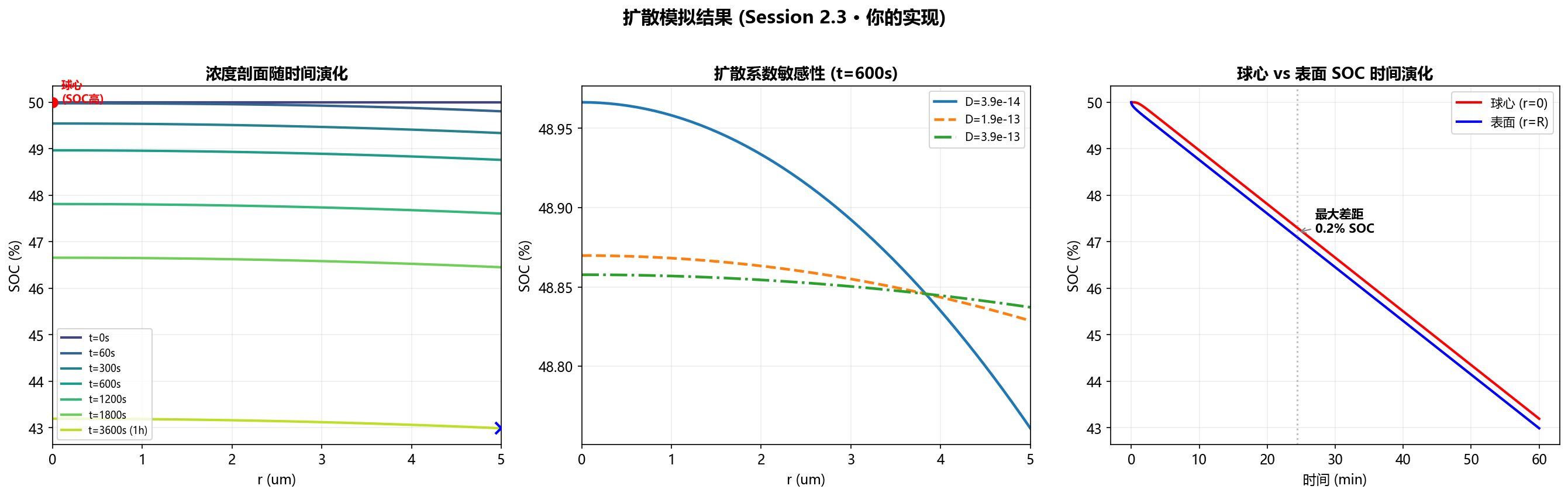
2.3.6 Simulation Result Figures

Left plot: concentration profiles from t=0 (uniform 50%) to t=3600s, surface SOC gradually decreases
Middle plot: larger D → flatter curves (verifying “larger diffusion coefficient = smaller concentration polarization”)
Right plot: center and surface SOC diverge — gap = degree of concentration polarization

III. Chapter Summary — Chapter 2 Complete Knowledge Map

3.1 All Formulas Learned

Formula	Meaning	Origin Session
$J = -D \cdot \partial c / \partial r$	Fick’s First Law	2.1
$\partial c / \partial t = D \cdot \partial^2 c / \partial r^2$	Fick’s Second Law (Cartesian)	2.1 hand-derived
$\partial c / \partial t = D \cdot [\partial^2 c / \partial r^2 + (2/r) \cdot \partial c / \partial r]$	Fick’s Second Law (spherical)	2.1
$c’(x) \approx (c_{i+1} - c_{i-1}) / (2dr)$	1st-order central difference	2.2 hand-derived
$c’’(x) \approx (c_{i+1} - 2c_i + c_{i-1}) / dr^2$	2nd-order central difference	2.2 hand-derived
$\nabla^2 c_i = \alpha_i c_{i-1} + \beta_i c_i + \gamma_i c_{i+1}$	Laplacian three-point difference	2.2 hand-derived
$\alpha_i = (1 - dr/r_i)/dr^2$, $\gamma_i = (1 + dr/r_i)/dr^2$	Spherical coordinate coefficients (via fraction combination)	2.2 hand-derived + breakdown when stuck
$\nabla^2 c	_0 = 6(c_1 - c_0)/dr^2$	Center Laplacian (3×2=6)
$D \cdot (c_{N-1} - c_{N-2}) / dr = j$	Surface Neumann boundary	2.2
$(I - D\Delta t \cdot L) \cdot c^{new} = c^{old}$	Implicit Euler matrix form	2.2 meaning of I
$\Delta t < dr^2/(2D) \approx 0.13\mathrm{s}$	Explicit CFL limit	2.2 hand-calculated

3.2 All Key Concepts

Concept	Intuitive Understanding	Session
Concentration c	How much Li per unit volume	2.1
Diffusion flux J	How many Li pass per second per unit area	2.1
Diffusion coefficient D	How fast Li “walks”	2.1
Concentration gradient ∂c/∂r	How steep the “slope” of concentration is	2.1
Spherical coordinate correction	Shell volume ∝ r² → geometric focusing	2.1
Concentration polarization	Surface dries out but interior still wet	2.1
Spatial discretization	Cutting continuous r into N points	2.2
Finite differences	Replacing derivatives with neighbor differences	2.2 hand-derived
Laplacian ∇²	The “diffusion operator” — how c diffuses at each point	2.2 hand-derived
Explicit vs. Implicit	Explicit is simple but unstable; Implicit needs matrix solve but unconditionally stable	2.2 CFL calculation
CFL condition	Maximum stable Δt for explicit methods	2.2 hand-calculated
Tridiagonal matrix	Only adjacent nodes are coupled → only 3 diagonals non-zero	2.2
L’Hôpital’s rule	Handling 0/0 at the center: differentiate numerator/denominator	2.2 hand-derived
Banded storage	Only storing non-zero diagonals, saving 94% memory	2.2
“Separation of static and dynamic”	Pre-build matrix, modify RHS each step — elegant design	2.3 code comparison

3.3 All Code Implementations

Function	Lines	Function	Key Technique
`build_diffusion_matrix()`	~25	Build (3, N) banded matrix	α_i, β_i, γ_i + if/elif/else three branches
`solve_one_step()`	~5	Execute one implicit Euler step	RHS injection j·dr/D + solve_banded
`simulate_diffusion()`	~15	Loop generate full time series	Pre-build ab, reuse per step (separation of static and dynamic)

3.4 Error/Bug Record

Bug	Cause	Fix
Banded storage index errors	ab column index confusion	ab[0,i+1], ab[1,i], ab[2,i-1]
Interior coefficients wrong	Forgot spherical correction α_i, γ_i	lam·alpha, lam·gamma
Surface RHS denominator wrong	Used r instead of D	`j * dr / D`
`NameError` c_history	Loop body was empty	Initialize c_history, assign each step

IV. Next Chapter Preview

Chapter 3: Butler-Volmer Kinetics — connecting current to overpotential η, completing the last piece of SPM’s full voltage chain.

Core formula:

$$
j = j_0 \cdot \left[ \exp!\left(\frac{\alpha F \eta}{RT}\right) - \exp!\left(-\frac{(1-\alpha)F \eta}{RT}\right) \right]
$$

Chapter 2 → Chapter 3 connection:

Diffusion Eq (Ch 2)              BV Kinetics (Ch 3)
      ↓                              ↓
  Provides c_s_surf  ──→  Computes overpotential η
      ↓                              ↓
      └──────────→  Voltage coupling V_cell  ←──────────┘

Study Notes · Part 2 Complete
Next: Part 3 — Butler-Volmer Kinetics

P2D Model Study Notes · Part 2: Diffusion Equation

Learning Method

Session 2.1: Physical Intuition — From “a Cup of Sugar Water” to the Spherical Coordinate Equation

2.1.1 What is Concentration?

2.1.2 Fick’s First Law — What Pushes the Sugar Molecules?

2.1.3 Fick’s Second Law — Hand-Derive from Mass Conservation

2.1.4 Spherical Coordinate Correction — The Onion Model

2.1.5 Two Boundary Conditions

2.1.6 Analogy — Spherical Sponge Squeezing

2.1.7 Session 2.1 Outputs

Extended Thinking (preview for Session 2.2)

Session 2.2: Numerical Methods — From Finite Differences to Tridiagonal Matrix

2.2.0 Warmup: Two Leftover Questions from Last Session

2.2.1 Spatial Discretization — Slicing the Particle into Points

2.2.2 Taylor Expansion → Finite Difference Hand-Derivation

2.2.3 Spherical Laplacian Discretization ⭐ Core Derivation

2.2.4 Explicit vs. Implicit Euler

2.2.5 Implicit Euler Matrix Form — What are I and L?

2.2.6 Center Boundary — Full L’Hôpital’s Rule Hand-Derivation

2.2.7 Surface Boundary + scipy Banded Storage

2.2.8 Session 2.2 Outputs

Extended Thinking (preview for Session 2.3)

Session 2.3: Code Practice — Write a Diffusion Solver from Scratch

2.3.0 Learning Method

2.3.1 Task 1: build_diffusion_matrix

2.3.2 Task 2: solve_one_step

2.3.3 Task 3: simulate_diffusion

2.3.4 Numerical Verification

2.3.5 Code Comparison Analysis

2.3.6 Simulation Result Figures

III. Chapter Summary — Chapter 2 Complete Knowledge Map

3.1 All Formulas Learned

3.2 All Key Concepts

3.3 All Code Implementations

3.4 Error/Bug Record

IV. Next Chapter Preview

2.3.1 Task 1: `build_diffusion_matrix`

2.3.2 Task 2: `solve_one_step`

2.3.3 Task 3: `simulate_diffusion`